How well do finite metric spaces embed in Euclidean space?
Abstract
Bourgain proves that every metric space with \(n\) points embeds in Euclidean space with distortion \(O(\log n)\), and constructs, from random graphs, metric spaces for which every embedding has distortion at least a constant multiple of \(\log n/\log\log n\). The lower bound shows in particular that \(O(\sqrt{\log n})\) is not achievable, and answers negatively a question of Johnson and Lindenstrauss (1984) about embeddings into normed spaces of dimension \(\log n\). The embedding sends each point to its distances from random sets of points of every size up to \(n\), and the analysis rests on a single estimate of how often such a set separates two given points. The theorem became a cornerstone of the theory of low-distortion embeddings of finite metric spaces. A decade later, Linial, London and Rabinovich (1995) made the construction algorithmic and proved that expander graphs require distortion of order \(\log n\), so that Bourgain's bound is best possible; with the independent work of Aumann and Rabani (1998), this made the embedding a basic tool of approximation algorithms, beginning with the sparsest cut problem.
Introduction
Let \((X,d)\) be a metric space with \(n\) points, for instance a connected graph with its shortest-path metric.1 We look for a map \(\emb\) from \(X\) into some Euclidean space (aside) \(\mathbb R^m\) such that \(\|\emb(x)-\emb(y)\|\) is as close to \(d(x,y)\) as possible for all \(x,y\in X\).
Bourgain writes Hilbert space instead. For finite spaces the two questions are the same: \(n\) points of a Hilbert space span a subspace of dimension at most \(n-1\), and that subspace is a copy of \(\mathbb R^k\) with its usual distance for some \(k\le n-1\).
Ideally \(\emb\) would be an isometry, that is, with all distances exactly preserved, \(\|\emb(x)-\emb(y)\|=d(x,y)\) for all \(x,y\). However, a space with as few as four points already rules this out.
Example 1: Four points
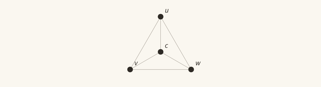
Let \(X\) consist of four points \(c,u,v,w\), where \(c\) is at distance \(1\) from each of \(u,v,w\) and these three are pairwise at distance \(2\) (left panel of Figure 1).
An isometry of this space would satisfy \(\|\emb(c)-\emb(u)\|+\|\emb(c)-\emb(v)\|=\|\emb(u)-\emb(v)\|\). Equality in the triangle inequality forces \(\emb(c)\) to be the midpoint of \(\emb(u)\) and \(\emb(v)\). By the same argument it is the midpoint of \(\emb(u)\) and \(\emb(w)\), so \(\emb(v)=\emb(w)\), contradicting \(d(v,w)=2\) (right panel of Figure 1).
Since even simple spaces do not admit isometries, we measure how far a map is from one. A map \(\emb\) may stretch some distances and shrink others, and we define its distortion as the largest stretch times the largest shrink,
(1)
The distortion is at least \(1\), does not change when \(\emb\) is rescaled, and equals \(1\) exactly when \(\emb\) preserves all distances up to a common factor. The best embedding of Example 1 places \(u,v,w\) at the corners of an equilateral triangle with \(c\) at its center (Widget 2); its distortion is \(2/\sqrt3\).

No dimension does better. Let \(c',u',v',w'\) be any four points of \(\mathbb R^m\) and let \(g\) be the centroid of \(u',v',w'\). Expanding the squares shows that
(2)
and since the centroid minimizes the sum of squared distances to the three points, the right side is at most \(3\bigl(\|u'-c'\|^2+\|v'-c'\|^2+\|w'-c'\|^2\bigr)\). Nothing in its proof depends on \(m\). Now take an embedding \(\emb\) of distortion \(\dst\), rescaled so that it shrinks no distance and preserves at least one, and apply the inequality to the images of \(c,u,v,w\). The images of each pair of leaves are at least \(2\) apart, so the left side is at least \(12\); each spoke has length at most \(\dst\), so the right side is at most \(9\dst^2\). Hence \(\dst^2\ge 4/3\), that is, \(\dst\ge 2/\sqrt3\). Equality forces \(c\) to sit at the centroid of an equilateral triangle, which is the configuration of Widget 2.
1. A first embedding
We now return to an arbitrary \(n\)-point metric space \((X,d)\) and look for a map that works for every such space at once. The most natural candidate, due to Fréchet, uses the points of \(X\) themselves as reference points: it is the map \(\emb\colon X\to\mathbb R^n\) that sends \(x\) to the vector of its distances to all points of \(X\) (aside), \(\emb(x)=\big(d(x,a)\big)_{a\in X}\).
Fréchet observed that this map preserves distances exactly if one measures the distance between two vectors by their largest coordinate difference, so every finite metric space embeds isometrically into \(\mathbb R^n\) with the maximum norm. See Fréchet (1910).
For all \(x,y,a\in X\), the triangle inequality gives \(|d(x,a)-d(y,a)|\le d(x,y)\), so
(1.1)
and no distance is stretched by more than \(\sqrt n\). In the coordinate indexed by \(a=x\), the images of \(x\) and \(y\) differ by \(d(x,y)\), so no distance is shrunk. Hence every \(n\)-point metric space embeds in \(\mathbb R^n\) with distortion at most \(\sqrt n\). On the following space the Fréchet embedding comes close to this bound.
Example 1.1: Star
For \(n\ge3\), let \(X\) consist of a center joined to \(n-1\) peripheral points, the leaves, with the shortest-path metric: the center is at distance \(1\) from each leaf, and two leaves are at distance \(2\). Example 1 is the star with \(n=4\).
As Figure 1.1 shows, the Fréchet embedding of the star has distortion \(\sqrt{n/2}\), although the star itself embeds with distortion at most \(\sqrt2\), for instance by sending the leaves to orthonormal vectors and the center to the origin.
The star shows that the Fréchet embedding cannot do much better than \(\sqrt n\). Write \(\dst(n)\) for the smallest number such that every \(n\)-point metric space embeds with distortion at most \(\dst(n)\); so far we know only that \(\dst(n)\le\sqrt n\).
How small is \(\dst(n)\), that is, how small a distortion can we guarantee knowing nothing about a space but its number of points?
2. What a good embedding needs
The large distortion of the Fréchet embedding on the star of Example 1.1 has a simple explanation. Each of its coordinates records the distance to a single point of \(X\), and how many of these coordinates separate two points, that is, take values at them that differ by an amount comparable to their distance, depends heavily on the pair: the center and a leaf differ in all \(n\) coordinates, whereas two leaves differ in only two of them (Figure 1.1). As a result, the first pair is stretched \(\sqrt{n/2}\) times as much as the second.
The imbalance matters because, by the triangle inequality, each coordinate of \(\emb(x)-\emb(y)\) is at most \(d(x,y)\) in absolute value, so \(\|\emb(x)-\emb(y)\|^2/d(x,y)^2\) essentially counts the coordinates that separate \(x\) from \(y\). More precisely, consider a map \(\emb\colon X\to\mathbb R^m\) with coordinates \(\emb_i=\sqrt{w_i}\,g_i\), where the weights \(w_i\ge0\) add up to \(1\) and each \(g_i\colon X\to\mathbb R\) satisfies \(|g_i(x)-g_i(y)|\le d(x,y)\) for all \(x,y\in X\). Think of \(i\) as a random index, chosen with probability \(w_i\), and suppose that for every pair \(x,y\) the random coordinate satisfies \(|g_i(x)-g_i(y)|\ge\beta\,d(x,y)\) with probability at least \(\alpha\). Then
(2.1)
so the distortion of \(\emb\) is at most \(1/(\beta\sqrt\alpha)\). The Fréchet embedding, rescaled by \(1/\sqrt n\), has this form with equal weights \(w_a=1/n\), \(\beta=1\) and \(\alpha=2/n\), since every pair \(x,y\) is separated, by exactly \(d(x,y)\), in the coordinates indexed by \(x\) and by \(y\); the bound gives \(\sqrt{n/2}\), which is the distortion on the star.
To improve on the Fréchet embedding, we therefore look for coordinates that separate every pair of points, by an amount proportional to its distance, with a probability \(\alpha\) such that \(1/n=o(\alpha)\). By the bound above, the distortion is then \(o(\sqrt n)\).
3. Distances to random sets
One coordinate in the Fréchet embedding separates so few pairs because of how it is built. On the star of Example 1.1, the coordinate \(d(\cdot,a)\) separates two leaves only when \(a\) is one of them, because every other point is equally far from both. In general, \(d(\cdot,a)\) separates \(x\) from \(y\) only when \(a\) is noticeably closer to one of them than to the other, and a single point can be in that position for very few pairs. This suggests replacing the reference point by a reference set \(A\subseteq X\), spread out over the space, and measuring the distance to its nearest element. On the star, for instance, \(d(\cdot,A)\) separates two leaves whenever \(A\) contains exactly one of them, and a set that contains each point with probability \(\tfrac12\) does so half the time (Figure 3.1).
For a set \(A\subseteq X\) we put \(d(x,A)=\min_{a\in A}d(x,a)\), with the convention \(d(x,\emptyset)=0\). The triangle inequality shows, exactly as before, that \(|d(x,A)-d(y,A)|\le d(x,y)\), so the map \(x\mapsto d(x,A)\), used as one coordinate of an embedding, never stretches a distance.
It remains to decide which sets to use, and rather than choosing them cleverly we choose them at random. Fix a number \(p\) with \(0<p\le1\), and let \(A\) be the random subset of \(X\) obtained by including each point of \(X\) independently with probability \(p\). We call \(p\) the density of \(A\): on average, \(A\) contains a fraction \(p\) of the points of \(X\).
One random set gives only one coordinate, which cannot separate all pairs, so we take many. If \(A_1,\dots,A_N\) are independent copies of \(A\), consider the map \(\emb\colon X\to\mathbb R^N\) with coordinates \(d(\cdot,A_1)/\sqrt N,\dots,d(\cdot,A_N)/\sqrt N\); then
(3.1)
which for large \(N\) is close to the expected value \(\mathbb E\,\big(d(x,A)-d(y,A)\big)^2\). To avoid estimating the error in this approximation, we can obtain the expected value exactly. Since \(X\) has only finitely many subsets, we may instead consider the map \(\emb\) with one coordinate for every subset \(S\subseteq X\), namely \(\sqrt{\Pr[A=S]}\;d(\cdot,S)\). For this map
(3.2)
A map of this kind, with one coordinate for every subset, is the form Bourgain used, although he draws his random sets differently (see the note to Theorem 7.1); a sampled version with far fewer coordinates came later, and we return to it in Section 10. The number of coordinates plays no role in the distortion.
This map has the form described before (2.1), with weights \(w_S=\Pr[A=S]\) and functions \(g_S=d(\cdot,S)\), so the upper bound there applies; the lower bound will come instead from adding up separations over all scales, in Section 6. Since each term \(\big(d(x,S)-d(y,S)\big)^2\) is at most \(d(x,y)^2\) and the probabilities add up to \(1\), the map \(\emb\) stretches no distance at all, and all that remains to analyze is how much it shrinks distances.
For the star this construction already gives bounded distortion. Take \(p=\tfrac12\) and consider first the center \(c\) and a leaf \(u\), at distance \(1\). If \(c\in A\), then \(d(c,A)=0\) while \(d(u,A)\) is \(0\) or \(1\) with equal probability. If \(c\notin A\) but \(A\) contains some leaf, then \(d(c,A)=1\) while \(d(u,A)\) is \(0\) or \(2\), so the difference is \(1\). Finally, \(A\) is empty with probability \(2^{-n}\), and then both distances are \(0\). The average squared difference is therefore \(\tfrac12\cdot\tfrac12+\big(\tfrac12-2^{-n}\big)\cdot1=\tfrac34-2^{-n}\). A similar count for two leaves, at distance \(2\), gives an average squared difference of exactly \(\tfrac54\). The distortion is therefore
(3.3)
for every \(n\), so on stars the distortion is \(O(1)\).
Which density \(p\) should we choose, and how much does the best choice improve on the bound \(\dst(n)\le\sqrt n\)?
4. All densities at once
The density \(p\) in Section 3 has to be chosen, and a good choice depends on the size of the regions in which two points differ. The following space shows this most clearly.
Example 4.1: Nested clusters
Let \(L\ge1\) and let \(X\) consist of \(n=2^L\) points arranged in nested clusters: pairs, pairs of pairs, and so on, up to the whole space. If the smallest cluster containing two distinct points \(x,y\) has \(2^h\) points, we say that the pair is at level \(h\) and set \(d(x,y)=b^h\), where \(b>1\) is fixed (Figure 4.1).
This is a metric space, and in fact it satisfies the stronger inequality \(d(x,z)\le\max\{d(x,y),d(y,z)\}\) for all \(x,y,z\in X\), since the level at which \(x\) and \(z\) join is at most the larger of the levels at which each joins \(y\). Metric spaces with this property are called ultrametric, and every finite ultrametric space embeds in Euclidean space with distortion \(1\), as Lemin (1985) showed. Consequently, if the map of Section 3 has large distortion on this space, the fault lies with that map and not with the space.
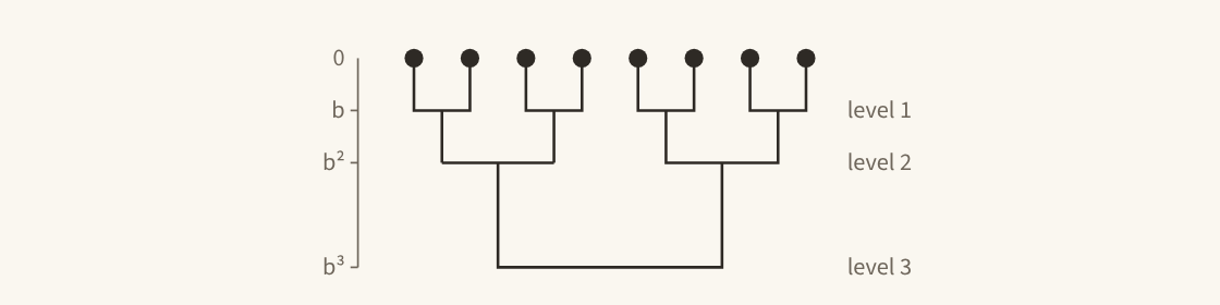

Consider a pair \(x,y\) at level \(h\). Their smallest common cluster splits into two halves of \(2^{h-1}\) points, one containing \(x\) and the other \(y\), and every point outside it is at the same distance from \(x\) as from \(y\). A random set of density \(p\) misses a given half with probability \((1-p)^{2^{h-1}}\) and so meets it with probability \(q=1-(1-p)^{2^{h-1}}\). The two halves are disjoint, so these events are independent, and the probability that \(A\) meets exactly one half is \(P_h(p)=2q(1-q)\).
Splitting according to which halves \(A\) meets (Widget 4.2), we can now bound the squared stretch of the pair, \(\|\emb(x)-\emb(y)\|^2/d(x,y)^2\), from below and from above:
(4.1)
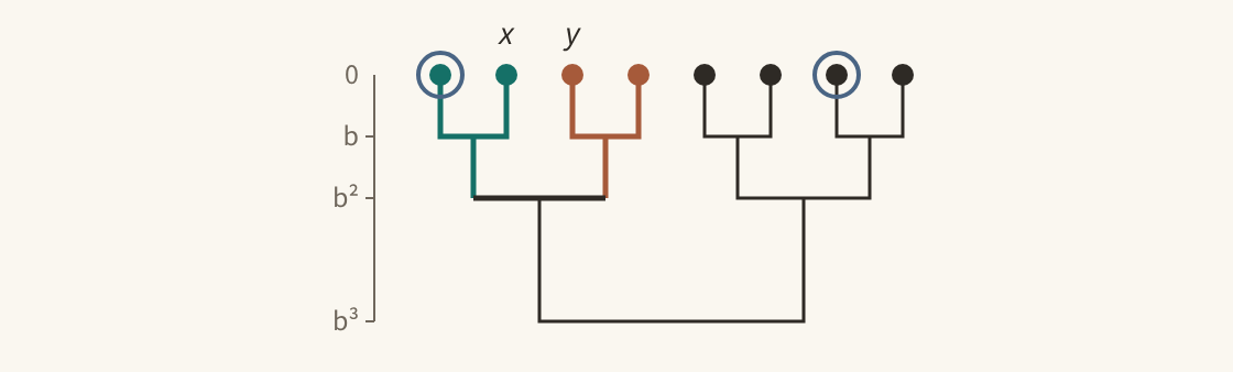
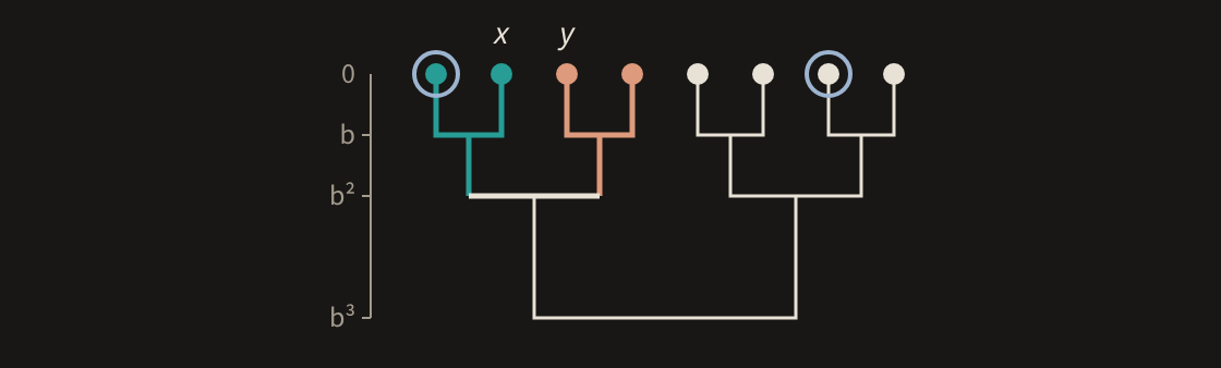
By (4.1), for large \(b\) the squared stretch of a pair at level \(h\) is essentially \(P_h(p)\), and no single density makes \(P_h(p)\) large at every level. For \(h=1\), \(P_1(p)=2p(1-p)\le2p\), which is small unless \(p\) is of order \(1\); for \(h=L\), \(P_L(p)\le2(1-p)^{n/2}\le2e^{-pn/2}\), which is small unless \(p=O(1/n)\). Meanwhile the level \(h\) with \(2^{h-1}\approx1/p\) has \(P_h(p)\) bounded below by a constant, so a density \(p\) serves the levels near \(h=1+\log_2(1/p)\) and few others (Widget 4.3, step 1). What decides whether a density separates a pair is therefore not the distance between the two points but the number of points around them: a random set of density \(p\) separates the pairs whose two halves each contain about \(1/p\) points. As \(b\to\infty\), the distortion of the map with density \(p\) on this space tends to \(\sqrt{\max_h P_h(p)/\min_h P_h(p)}\), so even the best single density gives a distortion that grows with \(n\), roughly like \(\sqrt{n/\log n}\) (aside), from about \(1.3\) at \(n=16\) to about \(5.2\) at \(n=1024\) (Widget 4.3, step 2).
The worst-served levels are the two ends, where \(P_1(p)\approx2p\) and \(P_L(p)\approx2e^{-pn/2}\). The best single density roughly balances them, which gives \(p\approx(2\ln n)/n\) and \(\min_hP_h(p)\approx(4\ln n)/n\), while \(P_h(p)\le\tfrac12\) at every level. The distortion is therefore of order \(\sqrt{n/\log n}\).
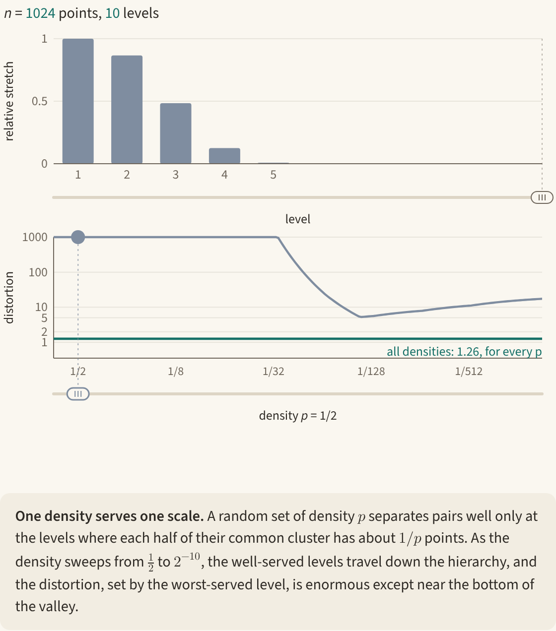
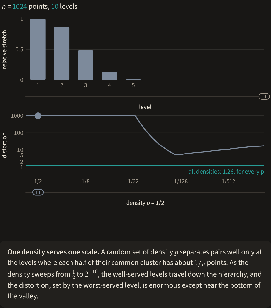
The computation also shows how to repair the construction. A pair at level \(h\) is well served by the density \(2^{-h}\): then \(q\) lies between \(1-e^{-1/2}\) and \(\tfrac12\), so \(P_h(2^{-h})\ge0.47\) for every \(h\). This suggests using all the densities \(\tfrac12,\tfrac14,\dots,2^{-L}\), where \(L=\lceil\log_2 n\rceil\), and to consider the map \(\emb\) obtained by placing the resulting maps side by side, so that
(4.2)
where \(\mathbb E_j\) denotes the expectation over random sets of density \(2^{-j}\). On the space of Example 4.1, let \(b\to\infty\) with \(n\) fixed; by (4.1), the squared stretch of a pair at level \(h\) tends to \(S_h=\sum_{j=1}^{L}P_h(2^{-j})\). Each \(S_h\) is at least \(0.47\), from the density \(2^{-h}\) alone, and at most an absolute constant, because \(P_h(2^{-j})\) falls off geometrically as \(j\) moves away from \(h\); so the distortion, \(\sqrt{\max_h S_h/\min_h S_h}\), stays bounded as \(n\) grows; numerically it is below \(1.3\) (Widget 4.3, step 3). In general, each of the \(L\) terms is at most \(d(x,y)^2\), so \(\emb\) stretches no distance by more than \(\sqrt L\). The rest of the argument shows that, in every finite metric space, \(\emb\) shrinks no distance by more than a factor \(O(\sqrt L)\).
5. One pair, one density
Section 4 showed that, on the space of Example 4.1, a random set of density \(p\) separates the pairs whose two halves each contain about \(1/p\) points, and there the halves are given by the hierarchy. A general metric space has no hierarchy, but the halves can be replaced by balls. Fix two distinct points \(x,y\in X\) and write \(\delta=d(x,y)\). For \(z\in X\) and \(r\ge0\) let \(B(z,r)\) be the closed ball of points at distance at most \(r\) from \(z\), and \(B^\circ(z,r)\) the open ball of points at distance less than \(r\). A random set of density \(2^{-j}\) has a constant chance of meeting a ball with at least \(2^{j-1}\) points and a constant chance of missing a ball with fewer than \(2^j\) points, so the scale at which this density can tell \(x\) from \(y\) is the radius at which the balls around them come to contain about \(2^j\) points.
Accordingly, for each integer \(j\ge0\) let \(r_j\) be the smallest radius \(r\) such that both \(B(x,r)\) and \(B(y,r)\) contain at least \(2^j\) points, with \(r_j=\infty\) if \(2^j>n\) (Widget 5.1). The radii start at \(r_0=0\) and never decrease as \(j\) grows. We use them only up to \(\delta/2\), setting \(\rad{j}=\min(r_j,\delta/2)\), and let \(k\) be the first index with \(\rad{k}=\delta/2\). Such an index exists and satisfies \(k\le L\): either \(2^L>n\) and \(r_L=\infty\), or \(2^L=n\) and each of the two balls of radius \(r_L\) contains all of \(X\), hence the other point, so that \(r_L\ge\delta\). The cap at \(\delta/2\) keeps balls around \(x\) and around \(y\) apart, which the proof below needs.
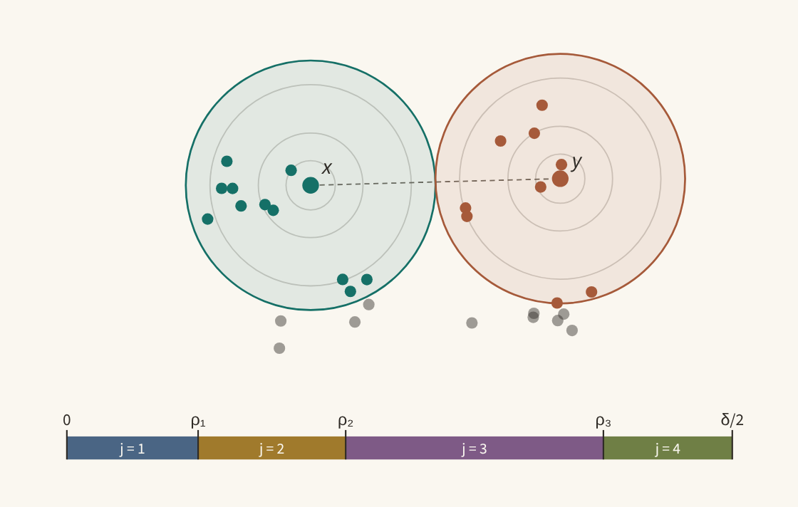
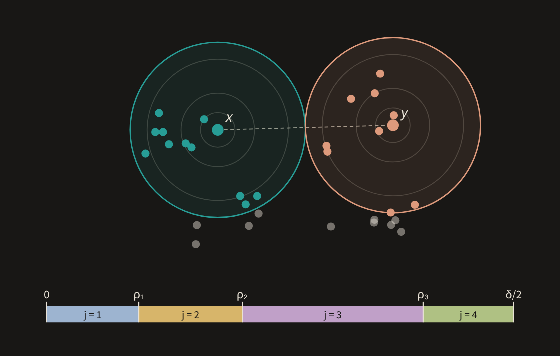
With these radii we can say what a single density achieves for the pair \(x,y\). The density \(2^{-j}\) is suited to the radii from \(\rad{j-1}\) to \(\rad{j}\), which form the \(j\)th segment of the bar in Widget 5.1, and the following lemma shows that it separates \(x\) from \(y\) by at least the length of that segment, with a probability that depends neither on \(j\), nor on the pair, nor on the space.
Lemma 5.1.
For each \(j\) with \(1\le j\le k\), a random set \(A\) of density \(2^{-j}\) satisfies \(|d(x,A)-d(y,A)|\ge\rad{j}-\rad{j-1}\) with probability at least \(c_0=(1-e^{-1/2})/e\approx0.145\).
Proof sketch.
Find a ball around one point that is large enough for \(A\) to hit and a ball around the other that is small enough for \(A\) to miss. The two balls are disjoint, so the two events are independent, and their probabilities depend only on point counts.
Proof of Lemma 5.1.
It SUFFICES to ASSUME \(\rad{j}>\rad{j-1}\).
Otherwise the required separation is at most \(0\).
⟨1⟩
⊢ Both \(B(x,\rad{j-1})\) and \(B(y,\rad{j-1})\) contain at least \(2^{j-1}\) points.
⟨2⟩
⊢ Exchanging \(x\) and \(y\) if necessary, \(B^\circ(y,\rad{j})\) has at most \(2^j-1\) points.
At any radius below \(r_j\) one of the two closed balls has fewer than \(2^j\) points, and since \(X\) is finite the same holds for one of the open balls of radius \(r_j\); if \(r_j=\infty\), every ball has fewer than \(2^j\) points. Finally \(\rad{j}\le r_j\).
⟨3⟩
⊢ \(B(x,\rad{j-1})\) and \(B^\circ(y,\rad{j})\) are disjoint.
A point in both would give \(\delta<\rad{j-1}+\rad{j}\le\delta\). This is where the cap at \(\delta/2\) is used.
⟨4⟩
⊢ If \(A\) meets \(B(x,\rad{j-1})\) and misses \(B^\circ(y,\rad{j})\), then \(|d(x,A)-d(y,A)|\ge\rad{j}-\rad{j-1}\).
On that event \(d(x,A)\le\rad{j-1}\) and \(d(y,A)\ge\rad{j}\).
⟨5⟩
⊢ \(A\) meets \(B(x,\rad{j-1})\) with probability at least \(1-e^{-1/2}\).
⟨6⟩
⊢ \(A\) misses \(B^\circ(y,\rad{j})\) with probability at least \(e^{-1}\).
⟨7⟩
Because each separation is the length of a segment of the bar in Widget 5.1, the separations add up: however unevenly the distance \(\delta/2\) is divided among the scales, the differences \(\rad{j}-\rad{j-1}\) for \(1\le j\le k\) sum to \(\rad{k}=\delta/2\). It is remarkable that the constant \(c_0\) is the same for every scale, every pair and every space: the probabilities in Step ⟨6⟩ and Step ⟨7⟩ involve only the counts \(2^{j-1}\) and \(2^j\) and the density \(2^{-j}\), so the geometry of \(X\) never enters, and this is what defining the radii by counting points was for.
Lemma 5.1 settles one pair and one density. How large is \(\|\emb(x)-\emb(y)\|\) for one pair and all densities?
6. One pair, all densities
We keep the pair \(x,y\) and the radii \(\rad{j}\) of Section 5, and now use all the densities together, through the map \(\emb\) of (4.2). Adding up the separations of Lemma 5.1 over the scales, we show that \(\emb\) shrinks the distance between \(x\) and \(y\) by at most a factor of order \(\sqrt L\).
The squared distance \(\|\emb(x)-\emb(y)\|^2\) is a sum of \(L\) terms, one for each density \(2^{-j}\), and the \(j\)th term is the expected value of \(\big(d(x,A)-d(y,A)\big)^2\) for a random set \(A\) of that density. Write \(a_j=\rad{j}-\rad{j-1}\) (aside).
The number \(a_j\) is the length of the \(j\)th segment of the bar in Widget 5.1.
\(\displaystyle \|\emb(x)-\emb(y)\|^2\ \ge\ c_0\sum_{j=1}^{k}a_j^2\)
For \(1\le j\le k\), Lemma 5.1 says that the square is at least \(a_j^2\) with probability at least \(c_0\), so the \(j\)th term is at least \(c_0a_j^2\); the remaining terms are nonnegative.
(6.1)
\(\displaystyle \ge\ \frac{c_0}{k}\Big(\sum_{j=1}^{k}a_j\Big)^2\)
A sum of squares with a given total is smallest when the summands are equal. The Cauchy–Schwarz inequality makes this precise, \(\big(\sum_{j=1}^k a_j\big)^2\le k\sum_{j=1}^k a_j^2\).
\(\displaystyle \ge\ \frac{c_0}{4L}\,d(x,y)^2 .\)
The lengths \(a_j\) add up to \(\delta/2\), but how this total is divided among them depends on the space, and \(k\le L\).
The map \(\emb\) therefore shrinks the distance between \(x\) and \(y\) by at most a factor \(2\sqrt{L/c_0}\). Nothing about the two points was used beyond their being distinct, and the factor depends on \(n\) alone.
7. Bourgain's theorem: all pairs, all densities
It remains to pass from one pair to all pairs and to combine the result with the stretch bound of Section 4; this gives Bourgain's theorem. Since the pair in Section 6 was arbitrary, (6.1) holds for all \(x,y\in X\), so \(\emb\) shrinks no distance by more than \(2\sqrt{L/c_0}\). By Section 4, it stretches no distance by more than \(\sqrt L\), because each of its \(L\) terms is at most \(d(x,y)^2\). Its distortion (1), the product of the two factors, is therefore at most
(7.1)
The two factors of \(\sqrt L\) have different origins. One is paid for having \(L\) densities, each of which may stretch a pair fully; the other is paid because, for a given pair, the separation may be spread thinly over all of them.
Recall from Section 1 that \(\dst(n)\) is the smallest number such that every \(n\)-point metric space embeds in Euclidean space with distortion at most \(\dst(n)\), and that the Fréchet embedding gives \(\dst(n)\le\sqrt n\). We have proved, with the explicit constant of (7.1), the following exponential improvement.
Theorem 7.1: Bourgain, 1985
\(\dst(n)=O(\log n)\); that is, every \(n\)-point metric space embeds in Euclidean space with distortion \(O(\log n)\).2
Is \(\log n\) the true order of \(\dst(n)\), or can every \(n\)-point metric space be embedded with distortion \(o(\log n)\)?
8. Bourgain's lower bound
Since \(\dst(n)\) bounds the distortion for all \(n\)-point spaces at once, a lower bound requires, for each \(n\), a single space that admits no embedding of small distortion. The claim concerns every embedding of that space, so it cannot be established by examining particular ones. Two methods establish it. The first, which goes back to Bourgain, is a counting argument: there are more essentially different spaces than embeddings of small distortion can tell apart. The second exhibits an inequality that every finite subset of Euclidean space satisfies and that the space violates by a large factor.
Bourgain's spaces come from sparse random graphs; the version presented here, due to Matoušek, uses graphs without short cycles. Fix an integer \(\ell\ge3\) and a graph \(G\) on \(n\) vertices with no cycle of length at most \(\ell\); such graphs exist with many edges3; let \(m\) be the number of edges of \(G\). Each of the \(2^m\) sets of edges of \(G\) spans a subgraph \(H\) on the same \(n\) vertices, and gives a metric space: the shortest-path distance in \(H\), truncated at \(\ell\) (Figure 8.1). For an edge \(uv\) of \(G\), the points \(u,v\) are at distance \(1\) if \(uv\) belongs to \(H\), and at distance \(\ell\) otherwise, since a path from \(u\) to \(v\) in \(H\) would close, with the edge \(uv\), a cycle of length greater than \(\ell\).
Suppose that all \(2^m\) of these spaces embed in Euclidean space with distortion at most \(\dst\), where \(\ell\ge8\dst\). By the Johnson–Lindenstrauss lemma (aside) the embeddings can be taken into \(\mathbb R^d\) with \(d\le C\log n\), at the cost of doubling the distortion; rescale each so that it stretches no distance and preserves at least one, and translate it into a ball of radius \(\ell\). Edges of \(G\) in \(H\) then have images of length at most \(1\), and the others images of length at least \(\ell/(2\dst)\ge4\). Now round every image point to the nearest point of a fixed set of at most \((8\ell)^d\) points that meets every ball of radius \(\tfrac12\) inside the ball of radius \(\ell\). Rounding moves each point by at most \(\tfrac12\), so it still shows, for every edge of \(G\), whether the edge belongs to \(H\), and different subgraphs give different rounded configurations. Counting both sides,
For every \(\varepsilon\in(0,1)\), any \(n\) points of a Euclidean space can be mapped into \(\mathbb R^d\) with \(d=O(\varepsilon^{-2}\log n)\) so that every distance changes by a factor between \(1-\varepsilon\) and \(1+\varepsilon\); a random linear projection does this with high probability, as Johnson and Lindenstrauss (1984) showed.
(8.1)
For the graphs chosen above, the left side of (8.1) is at least \(e^{(\ln n)/(\ell-1)}/9\), which exceeds the right side unless \(\ell\) is at least a constant multiple of \(\log n/\log\log n\). Taking \(\ell=\lceil8\dst\rceil\), it follows that if \(\dst\) is smaller than a suitable constant multiple of \(\log n/\log\log n\), then at least one of the \(2^m\) spaces has no embedding with distortion \(\dst\).
Theorem 7.1 and Theorem 8.1 determine \(\dst(n)\) up to a factor \(\log\log n\). Which of the two bounds gives its true order?
9. The sharp lower bound
The second method of Section 8 compares sums of squared distances over two sets of pairs. An inequality between two such sums that holds in every Euclidean space bounds from below the distortion of any metric space in which the pairs of the first set are much farther apart than those of the second. We first apply the method to the cube, where it gives \(\sqrt{\log n}\), and then to expander graphs, where it gives the sharp bound. We have already used one inequality of this kind, (2), to show that Example 1 needs distortion \(2/\sqrt3\). Another holds for any four points \(p_1,p_2,p_3,p_4\) of a Euclidean space:
(9.1)
which holds because the difference of the two sides is \(\|p_1-p_2+p_3-p_4\|^2\). In words, the diagonals of a quadrilateral are short compared with its sides. Applying it to the square faces of the cube \(\{0,1\}^k\) with the Hamming distance and inducting on \(k\) shows that every map \(\emb\) from the cube into a Euclidean space satisfies
(9.2)
where the left side runs over the \(2^{k-1}\) pairs of opposite vertices and the right side over the \(k2^{k-1}\) edges; for \(k=2\) this is (9.1). If \(\emb\) shrinks no distance, preserves at least one, and has distortion \(\dst\), each opposite pair, at distance \(k\), contributes at least \(k^2\) to the left side, and each edge at most \(\dst^2\) to the right side. Hence \(\dst\ge\sqrt k=\sqrt{\log_2 n}\) for \(n=2^k\), a result of Enflo (1969) and an early proof that \(\dst(n)\) is unbounded. The bound is only \(\sqrt k\) because the left side of (9.2) involves only the opposite pairs, one for every \(k\) edges. A bound of order \(\log n\) requires an inequality that involves almost all pairs, in a space where almost all pairs are far apart.
Expander graphs provide both. Let \(d\ge3\), let \(G\) be a connected \(d\)-regular graph on \(n\) vertices with the shortest-path metric, let \(\lambda_2\) be the second largest eigenvalue of its adjacency matrix \(M\), and write \(\gamma=d-\lambda_2\) for its spectral gap. The variational characterization of \(\lambda_2\)5, applied coordinate by coordinate, shows that every map \(\emb\) from the vertices into a Euclidean space satisfies
(9.3)
where the left side runs over all unordered pairs of distinct vertices. Rescale \(\emb\) so that it shrinks no distance and preserves at least one, and let \(\dst\) be its distortion. Each of the \(nd/2\) edges then has length at most \(\dst\), so the right side is at most \(n^2d\dst^2/(2\gamma)\). For the left side we count: at most \(d^{r+1}\) vertices lie within distance \(r\) of any given vertex, so choosing \(r+1=\lfloor\log_d(n/2)\rfloor\) leaves at least \(n^2/4\) pairs at distance at least \(r+1\). Comparing the two sides gives
(9.4)
For each fixed \(d\ge3\) there are \(d\)-regular graphs with arbitrarily many vertices whose spectral gap is bounded below by a positive constant depending only on \(d\); random \(d\)-regular graphs have this property with high probability. For them the bound (9.4) is \(\Omega(\log n)\), and together with Theorem 7.1 this settles the order of \(\dst(n)\).
Theorem 9.1: Linial, London and Rabinovich, 1995
10. After Bourgain
Once the worst case is settled, it is natural to ask which spaces do better. Trees are one such class: Matoušek (1999) showed that every \(n\)-vertex tree embeds with distortion \(O(\sqrt{\log\log n})\), and Bourgain (1986) showed, with complete binary trees, that this cannot be improved. Rao (1999) showed that planar graphs embed with distortion \(O(\sqrt{\log n})\), and Newman and Rabinovich (2003) that this is again best possible. For spaces of low dimension, measured by the doubling constant \(\lambda\), Krauthgamer et al. (2005) improved the bound to \(O(\sqrt{\log\lambda\cdot\log n})\), and Arora, Lee and Naor (2008) showed that finite subsets of \(\ell_1\) embed with distortion \(O(\sqrt{\log n}\,\log\log n)\).
A space that requires large distortion need not require it on most of its points. For every \(\varepsilon\in(0,1)\), every \(n\)-point metric space contains a subset of at least \(n^{1-\varepsilon}\) points that embeds with distortion depending only on \(\varepsilon\). This metric analogue of Ramsey's theorem is due to Bartal et al. (2005). Distortion also measures only the worst pair, and Abraham, Bartal and Neiman (2011) showed that the bound of Theorem 7.1 can be kept while the average distortion over all pairs is bounded by a constant.
The map of Section 7 has one coordinate for every subset of \(X\), and so exponentially many coordinates, but Linial, London and Rabinovich (1995) observed that \(O(\log n)\) random sets of each density already suffice with high probability, which brings the dimension down to \(O(\log^2 n)\) and turns the proof into an efficient randomized algorithm; the lemma of Johnson and Lindenstrauss (1984) reduces the dimension further to \(O(\log n)\), at the cost of a constant factor in the distortion. The same map embeds every \(n\)-point space into \(\ell_1\) with distortion \(O(\log n)\), and this algorithmic version gives an \(O(\log n)\) approximation for the sparsest cut problem in graphs, found independently by Linial, London and Rabinovich (1995) and Aumann and Rabani (1998).
Two questions close to Bourgain's theorem remain open. The first concerns finite subsets of \(\ell_1\), which by the result of Arora, Lee and Naor (2008) quoted above embed far better than general spaces. The cube \(\{0,1\}^k\) of Section 9 is such a subset, and Enflo's bound shows that its distortion is at least \(\sqrt{\log_2 n}\); it is not known whether this is the worst case.
Problem 10.1.
Does every \(n\)-point subset of \(\ell_1\) embed in Euclidean space with distortion \(O(\sqrt{\log n})\)?
A positive answer would remove the factor \(\log\log n\) from the bound of Arora, Lee and Naor. For subsets of \(\ell_p\) with \(p>2\), where the theorem of Section 7 had been the best available, Naor and Ren (2026) recently obtained distortion \((\log n)^{1/2+o(1)}\) for every fixed \(p\).
The second question concerns \(\ell_1\) as a target. Planar graphs need distortion of order \(\sqrt{\log n}\) in Euclidean space, but \(\ell_1\) accommodates more spaces, and Gupta et al. (2004) conjectured that in \(\ell_1\) a constant suffices for planar graphs and, more generally, for every family of graphs closed under taking minors other than the family of all graphs. They proved it for series-parallel graphs, and it has since been proved for several other special families, but for planar graphs the best known bound is still Rao's \(O(\sqrt{\log n})\).
Problem 10.2.
Is there a constant \(C\) such that every planar graph, with its shortest-path metric, embeds in \(\ell_1\) with distortion at most \(C\)?
The question we began with was how faithfully a finite metric space can be represented in Euclidean space. For the four points of Example 1 the answer is \(2/\sqrt3\); for \(n\) points it is of order \(\log n\).
The upper bound rests on a single idea, measuring distances to random sets of every density, so that each pair is separated at the scale where the points around it thin out. The lower bounds show that nothing substantially better is possible. Bourgain's own, by counting, comes within a factor \(\log\log n\) of the truth; the sharp one uses expanders, in which almost every pair is far apart, while in Euclidean space the inequality (9.3) keeps the average pair close relative to the edges.
The author chose the paper, directed the scope, structure, tone, depth and design of the presentation, reviewed every section, and checked the correctness of every argument. Claude Opus 5.5 (Anthropic) drafted much of the prose and built the interactive figures. Errors are the author's.